RESEARCH ARTICLE
Performance Analysis of an Optical System Using Dispersion Compensation Fiber & Linearly Chirped Apodized Fiber Bragg Grating
Vibha Joshi*, Rekha Mehra
Article Information

Identifiers and Pagination:
Year: 2016Volume: 3
First Page: 114
Last Page: 121
Publisher Id: PHY-3-114
DOI: 10.2174/1874843001603010114
Article History:
Received Date: 25/12/2015Revision Received Date: 29/5/2016
Acceptance Date: 08/9/2016
Electronic publication date: 31/10/2016
Collection year: 2016
open-access license: This is an open access article licensed under the terms of the Creative Commons Attribution-Non-Commercial 4.0 International Public License (CC BY-NC 4.0) (https://creativecommons.org/licenses/by-nc/4.0/legalcode), which permits unrestricted, non-commercial use, distribution and reproduction in any medium, provided the work is properly cited.
Abstract
In this paper, a proposal for analyzing the performance of an optical system by using dispersion compensation fiber (DCF) and linear chirped apodized fiber Bragg grating (FBG) has been put forth. Both systems have three different schemes pre, post and symmetrical. Various parameters used for this analysis are input power, distance & input bit rate. Performance is analyzed in terms of Q factor, Bit Error Rate (BER) and Eye Diagram. It is found that use of FBG as a dispersion compensating element gives better system performance as compared to DCF.
I. INTRODUCTION
Information in fiber optic communication system is transmitted in the form of light pulses from transmitter to receiver. The light is an electromagnetic carrier wave, which is modulated to carry information. Like other communication systems, optical communication system also faces problems such as dispersion, attenuation and non-linear effects that degrade its performance. Amongst them dispersion effect is dominant and is difficult to overcome in comparison of other problems [1].
Dispersion can be defined as broadening of light pulses in an optical fiber which decreases the data rates, signal to noise ratio and quality of the system. Dispersion causes broadening of pulses which leads to Inter-Symbol-Interference (ISI), in which the output pulses of a system overlaps. Due to this overlapping the output becomes undetectable. Thus, it is necessary to find out an effective dispersion compensation technique that leads to performance enhancement of the optical system [2].
Several dispersion compensation techniques available are- Dispersion shifted fibers, Dispersion-flattened fibers, all pass filters, raised cosine filter, high order mode fibers, DCF’s & Fiber Bragg Grating etc. [3].
Thyagarajan et al. presented a novel design of a dispersion compensating fiber [4]. Knudsen et al. shows optimization of dispersion compensating fiber for long haul applications [5]. Bo-ning HU et al. analyzed Fibres-optic dispersion and its effect on optical transmission system [6]. M. I. Hayee et al. presented the group velocity dispersion (GVD) and nonlinear effects, such as self- and cross-phase modulation (SPM/XPM) and four-wave mixing (FWM) in wavelength-division-multiplexed (WDM) systems at 10 Gb/s that degrade the performance of the system [7]. Luis Miguel Rio de Sousa Ramos et al. presented the characterization of fiber Bragg grating for dispersion compensation [8].
In this paper the performance of the system is measured in terms of Q factor, BER and Eye Diagram by varying the system parameters. The network layout is designed and simulated with the help of Optisystem 7 software. This paper is divided into V sections: Section II consists of theory, Section III deals with the system description including description of system parameters, Section IV shows the results & discussion and finally Section V concludes the paper.
II. THEORY
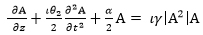
Avoiding polarization and scattering effects such as stimulated Raman scattering and stimulated Brillouin scattering, propagation of optical pulses in fiber is described by the scalar nonlinear Schrodinger’s equation (NLSE). It describes the evolution of optical field at the transmission distance z as [9, 10].
 |
(1) |
Where A represents the optical field envelope, γ is the nonlinearity coefficient, α is the attenuation constants θ1, θ2 and θ3 are first-order, second- and third-order derivations of the propagation constant θ about the center frequency ωο and they are related to the dispersion of the optical fiber, and TR can be related to the slope of the Raman gain spectrum and is usually estimated to be 3 femto-second at wavelengths near 1550 nm. The term proportional to θ3 account for third-order dispersion, and only becomes important for ultra short pulses, because of their wide bandwidth. The last two terms in the right side of the eqn. (1) are related to the effects of self-steeping and stimulated Raman scattering, respectively. For pulses of width To > 5 pico-second, the parameters 1/(ωο To) and TR/T0 become so small (< 0:001) that the last two terms in eqn. (1) can be neglected on such condition, and if the reference time frame moves with pulse at the group velocity, vg i.e. T = t - z/vg = t -θ1 z, the eqn. (1) can be simplified
 |
(2) |
The nonlinear effects included in the NLSE are self-phase modulation (SPM), cross-phase modulation (XPM), and four-wave mixing (FWM). Single channel transmission is affected by SPM only whereas multi channel transmission has combined effects of SPM, XPM, and FWM which lead to signal degradation. SPM affects the optical signal by its interaction with pulses broaden due to dispersion. Degradation due to nonlinear effect can be minimized by using appropriate dispersion compensation schemes [11]. Since dispersion of the SMF is large at 1550 nm (D = 16 ps / (nm.km)), thus it becomes necessary to compensate dispersion. Two compensation techniques used for this are as follows:
a. Dispersion Compensating Fiber
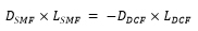
Dispersion compensating fiber is a single mode fiber which have high negative dispersion coefficient of -80 to -90 ps (nm.km)-1, and used to mitigate the positive dispersion of the single mode fiber. Its effective core area is small compared to single mode fiber and have high attenuation coefficient. The lengths of DCF and SMF are in the multiple of 1:5. By placing one DCF with negative dispersion after or before a SMF with positive dispersion, the net dispersion can be minimized or made equals to zero. The condition that makes net dispersion zero is
 |
(3) |
Where DSMF and LSMF are the dispersion and length of single mode fiber and DDCF and LDCF are the dispersion and length of dispersion compensating fiber.
b. Fiber Bragg Grating
Fiber Bragg gratings were introduced in 1980. These gratings are used in an optical fiber as a reflective device in which modulation of core refractive index takes place at a certain wavelength. The reflection occurs in gratings when the wavelength of signal travelling inside the optical fiber matches to the modulation periodicity of FBG. The reflected wavelength (λb) is known as the Bragg wavelength, and it is represented by the following relationship:
 |
(4) |
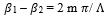
Where neff represents the effective refractive index of the grating in the fiber core and Λ represents the grating period. The operation of fiber Bragg grating depends on parameters such as: the reflection of light from grating fringes and on the coupling of the modes [11]. The coupling takes place between the forward and backward propagating fields. According to the coupling process, the two fields show strong coupling if they follow the given Bragg condition:
 |
(5) |
Where, β1 and β2 are the phase constants of two coupling modes, Λ depicts the grating period based on variation of the refractive index (assuming sinusoidal variation), and m is the order of diffraction. For first order, m =1.
Taking identical two inverse propagating modes
 |
(5) |
From equation (5) the Bragg diffraction condition becomes
 |
(7) |
On substituting the value of grating period Λ from equation (4) to (7), we get [12]
 |
(8) |
The chirped fiber Bragg grating is shown in Fig. (1).
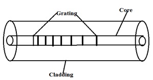 |
Fig. (1). Chirped fiber bragg grating [12]. |
Gratings which have non uniform period along their length in FBG are termed as Chirped Gratings. The chirp may be linear, may be quadratic, or may even have jumps in the period. A grating could also have a period that varies in any function along its length. Apodization causes the reduction of side-lobe levels in the reflection spectrum [13].
III. SYSTEM DESCRIPTION
For analyzing the system performance with DCF & FBG respectively the schematic experimental setup is shown in Fig. (2a-c). In this, data transmitter comprises of continuous wave laser operated at 193.1THz frequency or approximate 1550nm wavelength with output power of 5 dBm. The pulse train is intensity modulated with pseudo random bit sequence generator which uses bit rate of 10Gbps. This 10Gbps signal is encoded by pulse generator with the 0.5 duty cycle and then combine at Mach-Zehnder modulator with 30 dB of extinction ratio and modulated signal is then transmitted over channel. Channel is designed by single mode fiber, either DCF or FBG and optical amplifier with the length 5m.DCF & SMF have lengths in the multiple of 1:5. DCF have effective core area of 30µm2 .Similarly FBG also has certain parameters which are as follows: The length of the grating is used of 6mm. Apodization profile is hyperbolic tangent and linear chirp is being used. Both of these profiles have minimum side lobes [14]. After dispersion compensation the signal will pass through an optical amplifier. Optical amplification is required to overcome the fiber loss and it also amplifies the signal at the receiver port. The overall link is operated at 1550nm wavelength. At the receiver, optical signal is detected by photodiode with responsitivity 1[A/W]. Finally the signal is fed to BER analyzer to generate Eye diagram, Q-factor, and BER.
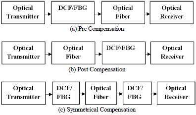 |
Fig. (2). Dispersion compensation schemes. |
According to the relative position of DCF or FBG with single mode fiber pre, post and symmetrical techniques are proposed. In Pre compensation DCF or FBG is placed before a single mode fiber or after the optical transmitter. Post compensation scheme is achieved by placing the DCF or FBG after a SMF or before the optical receiver. Symmetrical (Symm) or Mix compensation is the combination of pre and post compensation.
IV. RESULTS AND DISCUSSION
The simulation results have been compared for various compensation schemes. Various parameters have been used for this analysis are distance, input power and input bit rate. Performance can be measured in terms of Q factor, BER and Eye Diagram.
Tables 1 and 2 display the effect of variation in fiber length in terms of Q-Factor & BER. As the fiber length increases, Q factor decreases & BER increases. In case of equal fiber length, the value of quality factor varies for different compensation techniques. Fig. (3a and b) represent the eye diagrams of the two systems.
| LENGTH (Km) | DCF PRE | FBG PRE | DCF POST | FBG POST | DCF SYMM | FBG SYMM |
|---|---|---|---|---|---|---|
| 5 | 45.2005 | 223.822 | 78.462 | 260.772 | 80.2322 | 320.738 |
| 10 | 24.390 | 109.517 | 50.0041 | 109.315 | 60.2839 | 269.221 |
| 15 | 14.714 | 56.2247 | 47.3037 | 61.8682 | 12.1566 | 126.435 |
| 20 | 20.288 | 25.3462 | 20.988 | 32.5762 | 7.9788 | 78.5257 |
| 25 | 17.036 | 19.9368 | 9.76486 | 24.5826 | 6.17394 | 53.4323 |
| 30 | 20.223 | 8.6172 | 9.70943 | 24.217 | 5.97851 | 33.3471 |
| LENGTH (Km) | DCF PRE | FBG PRE | DCF POST | FBG POST | DCF SYMM | FBG SYMM |
|---|---|---|---|---|---|---|
| 5 | 0.0000000E+00 | 0.0000000E+00 | 0.0000000E+00 | 0.0000000E+00 | 0.0000000E+00 | 0.0000000E+00 |
| 10 | 5.5539300E-132 | 0.0000000E+00 | 0.0000000E+00 | 0.0000000E+00 | 0.0000000E+00 | 0.0000000E+00 |
| 15 | 1.7451700E-40 | 0.0000000E+00 | 0.0000000E+00 | 0.0000000E+00 | 1.3497400E-34 | 0.0000000E+00 |
| 20 | 7.1810300E-92 | 3.6689200E-142 | 2.2567100E-98 | 4.3174600E-233 | 7.2709200E-16 | 0.0000000E+00 |
| 25 | 1.7999800E-65 | 8.1989800E-89 | 4.1848300E-23 | 9.0540600E-134 | 3.0516800E-11 | 0.0000000E+00 |
| 30 | 2.5051100E-91 | 1.9351600E-18 | 8.5952600E-23 | 7.2240800E-130 | 9.4386000E-10 | 3.4093100E-244 |
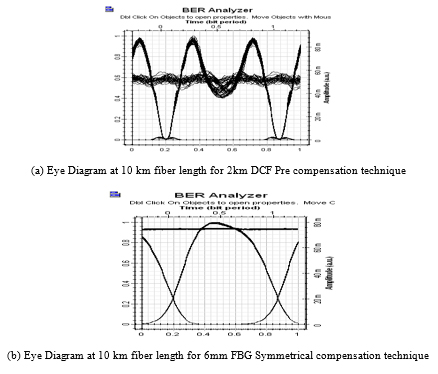 |
Fig. (3). Simulation results for different compensation schemes at different fiber length. |
Tables 3 and 4 represent the effect of variation in input power. The effect of laser power is contrary to the effect of fiber length. As the input power increases Q factor also increases and BER decreases in some configurations but due to non linearity effect it is not true for all the configurations. Fig. (4a and b) indicate the eye diagrams of the two systems.
| POWER (dBm) | DCF PRE | FBG PRE | DCF POST | FBG POST | DCF SYMM | FBG SYMM |
|---|---|---|---|---|---|---|
| 1 | 25.0502 | 109.124 | 45.7851 | 108.564 | 51.2178 | 256.11 |
| 5 | 24.3904 | 109.517 | 50.0041 | 109.315 | 60.2869 | 269.221 |
| 10 | 22.975 | 112.256 | 45.1231 | 106.551 | 63.6355 | 268.237 |
| 15 | 21.7493 | 116.196 | 35.9435 | 105.496 | 38.4011 | 252.288 |
| 20 | 13.7311 | 120.264 | 18.3551 | 122.463 | 10.8894 | 298.118 |
| POWER (dBm) | DCF PRE | FBG PRE | DCF POST | FBG POST | DCF SYMM | FBG SYMM |
|---|---|---|---|---|---|---|
| 1 | 4.54600 E-139 | 0.0000000E+00 | 0.0000000E+00 | 0.0000000E+00 | 0.0000000E+00 | 0.0000000E+00 |
| 5 | 5.55300 E-132 | 0.0000000E+00 | 0.0000000E+00 | 0.0000000E+00 | 0.0000000E+00 | 0.0000000E+00 |
| 10 | 2.11000 E-117 | 0.0000000E+00 | 0.0000000E+00 | 0.0000000E+00 | 0.0000000E+00 | 0.0000000E+00 |
| 15 | 1.85100 E-105 | 0.0000000E+00 | 1.6504800E-283 | 0.0000000E+00 | 3.45846E-23 | 0.0000000E+00 |
| 20 | 1.68380 0E-43 | 0.0000000E+00 | 9.1083700E-76 | 0.0000000E+00 | 3.2875400E-28 | 0.0000000E+00 |
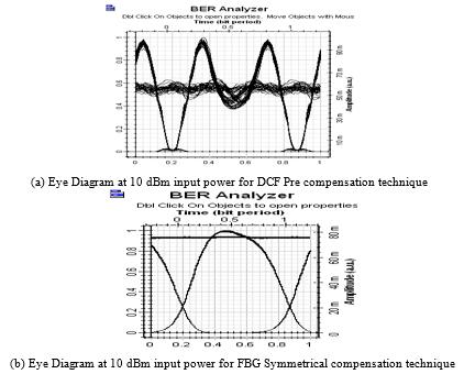 |
Fig. (4). Simulation results for different compensation schemes at different input power. |
Tables 5 and 6 display the effect of variation in input bit rate in terms of Q-Factor & BER. This also indicates that as the bit rate increases, quality of system decreases. Fig. (5a and b) represent the eye diagrams of the two systems.
| BIT RATE | DCF PRE | FBG PRE | DCF POST | FBG POST | DCF SYMM | FBG SYMM |
|---|---|---|---|---|---|---|
| 2.5 | 50.5586 | 244.016 | 102.513 | 181.765 | 107.384 | 764.05 |
| 5 | 29.307 | 160.285 | 61.3955 | 133.87 | 63.9906 | 398.234 |
| 10 | 24.3904 | 109.517 | 50.0041 | 109.315 | 60.2869 | 269.221 |
| 20 | 11.4093 | 28.54 | 17.2627 | 35.0933 | 9.2257 | 14.3201 |
| 30 | 3.32346 | 10.8868 | 10.1764 | 6.50373 | 7.7794 | 3.48195 |
| 40 | 3.10637 | 3.24516 | 6.39088 | 2.89819 | 4.18212 | 1.92539 |
| BIT RATE | DCF PRE | FBG PRE | DCF POST | FBG POST | DCF SYMM | FBG SYMM |
|---|---|---|---|---|---|---|
| 2.5 | 0.0000000E+00 | 0.0000000E+00 | 0.0000000E+00 | 0.0000000E+00 | 0.0000000E+00 | 0.0000000E+00 |
| 5 | 1.9294100E-189 | 0.0000000E+00 | 0.0000000E+00 | 0.0000000E+00 | 0.0000000E+00 | 0.0000000E+00 |
| 10 | 5.5539300E-132 | 0.0000000E+00 | 0.0000000E+00 | 0.0000000E+00 | 0.0000000E+00 | 0.0000000E+00 |
| 20 | 1.2085300E-30 | 1.6366000E-179 | 2.6974100E-67 | 3.7817100E-270 | 7.5058600E-21 | 5.3676200E-47 |
| 30 | 2.5539800E-04 | 5.6309600E-28 | 8.4588600E-25 | 3.3405800E-11 | 2.4507800E-15 | 1.8919000E-04 |
| 40 | 6.4414900E-04 | 4.6195800E-04 | 7.8183300E-11 | 1.6144900E-03 | 1.2538700E-05 | 2.2467000E-02 |
 |
Fig. (5). Simulation results for different compensation schemes at different input bit rate. |
From all the simulation results, one can attribute that symmetrical compensation with fiber Bragg grating provides excellent dispersion compensation. By visualizing the eye diagram it indicates that the signal quality is high, Eye shape is satisfactory. The Larger the Eye opening, the bigger will be Q factor with smaller BER. This indicates that use of FBG improves the eye diagram.
Fiber Bragg grating has simple structure, low insertion loss, high wavelength selectivity, polarization insensitivity and compatibility with optical fiber. Dispersion Compensation Fiber has high negative dispersion which is achieved by the shrinking of core diameter. A fiber with small core diameter experiences high light intensity and suffers from the high level of nonlinearity effects. Tables 1 and 2 show that BER is directly proportional to the fiber length. When fiber length increases, the Q factor decreases. Tables 3 and 4 indicate that rise in input power also gives rise to Quality factor in some configurations but due to non linearity effect it is not true for all the configurations. Similarly, Tables 5 and 6 represent that increase in the bit rate, causes reduction in Quality factor. Overall the performance of fiber Bragg grating in optical communication system is better than Dispersion Compensation Fiber.
CONCLUSION
In this paper, performance of an optical communication system has been analyzed by using DCF and FBG. The analysis was conducted on the basis of results observed from Optisystem simulation tool. In this analysis various parameter were used i.e. distance, input power & input bit rate. In all three schemes (pre, post & symmetrical) of FBG based system, if the length of fiber increases, it causes decrease in quality factor whereas a decrement in BER is observed on increasing the input power. On the other hand increase in input bit rate reduces the quality factor of the FBG based system. On comparing all the three schemes it was found that the FBG symmetrical scheme gives optimum results. Similarly in these schemes of DCF based system on increasing the length of fiber there is a decrease in quality factor whereas a decrease in BER is observed on increasing the input power. It was also found that as the input bit rate increases it reduces the quality factor of the system. Among all the three schemes (pre, post & symmetrical), DCF symmetrical scheme gives best results. On comparing both the systems; one with DCF and other with FBG it can be concluded that FBG symmetrical scheme results in better system performance.
CONFLICT OF INTEREST
The authors confirm that this article content has no conflict of interest.
ACKNOWLEDGEMENTS
Declared none.