RESEARCH ARTICLE
Mechanical Resonance Dispersion Revisited
Haskell V. Hart*
Article Information
Identifiers and Pagination:
Year: 2014Volume: 1
First Page: 1
Last Page: 14
Publisher Id: PHY-1-1
DOI: 10.2174/1874843001401010001
Article History:
Received Date: 2/7/2014Revision Received Date: 23/8/2014
Acceptance Date: 25/8/2014
Electronic publication date: 31/12/2014
Collection year: 2014
open-access license: This is an open access article licensed under the terms of the Creative Commons Attribution Non-Commercial License (http://creativecommons.org/licenses/by-nc/3.0/) which permits unrestricted, non-commercial use, distribution and reproduction in any medium, provided the work is properly cited.
Abstract
Mechanical resonance dispersion is the inelastic response of a solid to a periodic shear stress. Instead of the elastic Young's Modulus, the phenomenon is described by both a real J', and an imaginary J'' component of complex shear compliance, corresponding to in phase and out of phase strain responses, respectively. The experimental results are plots of J' and J'' vs. frequency, which are typically in the audiofrequency range of 10 - 5600 Hz. Resonances are observed as maxima in J'' and inversions in J' at frequencies corresponding to modes of plastic deformation, which are much lower frequencies (audiofrequency range) than elastic normal modes. The theoretical explanation of Edwin R. Fitzgerald involves particle waves and momentum transfer and leads to a particle-in-a-box frequency formula for these inelastic modes. Unfortunately, most of his and other published raw data were never analyzed by this model. The purpose of this article is to apply this formula to previously uninterpreted resonance dispersion curves and to address some of the earlier criticism of Fitzgerald's work. Results of these calculations support the Fitzgerald Theory to a high degree, demonstrate the importance of impurities and chemical analysis, largely mollify previous criticisms, and suggest the possibility of a new particle wave mass spectroscopy at great distances.
1. INTRODUCTION
Mechanical resonance dispersion (MRD) has been applied to such diverse systems as whale blubber [1], violin wood [2], human cancellous bone, natural rubber, synthetic polymers, and a variety of single crystal and polycrystalline solids, both elements and compounds (other references below in context), with the goal of understanding the mechanical response of the solid to periodic stress in the audiofrequency range. According to Edwin R. Fitzgerald [3], the complex (hence "dispersion") shear compliance, J*=J'-iJ'', with J' equal to the (energy) storage compliance and J'' equal to the (energy) loss compliance. This is the manifestation of a periodic shear stress, α, resulting in a periodic strain, a, with both in phase and out of phase components: a = s0
In a typical Fitzgerald experiment [3], the sample disk is clamped between piezoelectric transducers and is subjected to periodic shear stress at specific narrowly spaced frequencies. J' and J" are calculated at each frequency from knowledge of the electrical circuit [1], yielding a "spectrum" for a particular material. The details of the spectrum are a function of the chemical composition, including impurities, the crystallinity, the previous processing (e.g., sintering, fusion, quenching, or annealing), and to a lesser extent the static stress on the sample and the duration of the experiment.
2. COMPUTATIONAL METHODS
The classical mechanical model predicts a single resonance frequency, but nearly all spectra, including those of elements, show multiple resonances. To explain these and other details, Fitzgerald [4] invoked a momentum transfer equation for a one dimensional lattice of N atoms (1, 2, ...N) of mass m and velocities, v1,v2,...,vn-1,vnvn-1,...vN,,
where Kp is the momentum transfer constant, found to be equal to , with h equal to Planck's Constant, m the atomic mass, and d the interatomic spacing.
Applying boundary conditions to standing particle wave solutions to (1), the Planck-Einstein Equation, E = hv, plus the deBroglie Relation, pλ = h, Fitzgerald derived the particle-in-a-box normal mode frequencies
from which we obtain the operational equation for interpreting MRD spectra,
Here S equals Nd, the crystal mosaic size, and q a quantum number 1, 2, ... N-1. A standing particle wave is thus fixed between the endpoints of the mosaic separated by S and can have N-1 wavelengths from 2S to 2d. Since momentum is conserved in each of three dimensions, Eq. (1) is applicable to any row of like atoms in a crystal. An identical result, Eq. (2), was obtained [4, 5] by applying the time-dependent Schrödinger Equation.
For many materials a common dimension for crystal mosaics is on the order of 1 μm. This adds a further criterion for correct spectral assignments according to Eq. (3):S ≃ 1 μm. Of course, elements chosen, which determine m, must be known to be present in the sample or likely to be present based on sample origin and history.
Interpretation of a spectrum of resonance frequencies by this model will consist of choosing an element or an isotope for a highly resolved spectrum and a value of q for each resonant frequency such that a common value of S is calculated by Eq. (3) for all resonant frequencies in the spectrum.
This has been done only rarely previously for multiple resonances [6-9] where frequency series with ratios 1: 4: 9: 16…q2 were found (twice retrospectively). Such a complete spectrum is not observed in any of the 38 spectra interpreted below, and never without additional resonances, hence the need to identify previously unrecognized sample impurities in the large majority of MRD spectra. The purpose of this article is to apply this formula (Eqs. (2) and (3)) to previously uninterpreted MRD spectra and to address some of the earlier criticism of Fitzgerald's work.
Experimental resonant frequencies V listed in the following tables were either specifically mentioned in text or tables by the authors of the respective references or were taken from their spectra figures by this author. Eq. (3) was used to calculate S from each frequency and the assigned values of atomic or isotopic mass and q. The average value of S, Sav, for each sample was used to calculate Vc from Eq. (2) for comparison with experimental values, V. Throughout the following tables, an element symbol implies no resolution of isotopes or a monoisotopic element and the use of the atomic weight [10] in determining m for Eq. (3). A specific isotope designation implies use of the specific isotopic mass [11] in Eq. (3).
3. RESULTS AND DISCUSSION
3.1. Metals
3.1.1. Elemental
Table 1 lists data [3] from three different polycrystalline lead samples cut from the same bar. Samples A and C have the same dimensions, but were cut from different ends of the bar. Sample B was cut near A but had different dimensions.
Polycrystalline leada, Ref. [3].
| Isotope/Element | v(Hz) | vc(Hz) | q | S(µm) |
|---|---|---|---|---|
| Sample A | ||||
| 44Ca | 975 | 977 | 1 | 1.08 |
| Ag | 1600 | 1592 | 2 | 1.08 |
| Pb | 1850 | 1865 | 3 | 1.08 |
| OR Bi | 1849 | 3 | 1.08 | |
| 65Cu | 2650 | 2645 | 2 | 1.08 |
| 60Ni | 2875 | 2866 | 2 | 1.08 |
| Sample A Annealed | ||||
| Cu | 2900 | 2904 | 2 | 1.04 |
| Pb | 3550 | 3363 | 4 | 1.04 |
| OR Bi | 3532 | 4 | 1.04 | |
| Sample Bb | ||||
| Cu | 2825 | 2852 | 2 | 1.05 |
| Pb | 3500 | 3498 | 4 | 1.05 |
| OR Bi | 3469 | 4 | 1.04 | |
| Sample B Annealed | ||||
| Pb | 3550 | 3563 | 4 | 1.04 |
| OR Bi | 3532 | 4 | 1.04 | |
| Sample Cc | ||||
| 65Cu | 2815 | 2887 | 2 | 1.04 |
| Pb | 3650 | 3619 | 4 | 1.03 |
| OR Bi | 3588 | 4 | 1.02 | |
a Chemical analysis: Bi<0.0001%, Cu 0.0001%, Fe 0.0002%
b Different dimensions
c Obtained from different location on bar, dimensions same as Sample A.
The importance of trace impurities (Cu, Ag, Ca, Ni and possibly Bi) is made strikingly obvious by this interpretation. Resonances due to copper were the strongest. Silver, a common lead impurity, was not reported in the chemical analysis, but is indicated based on a weak resonance. Lead and bismuth resonances would probably not have been resolved, so both possibilities are listed. In the Betterton-Kroll refining process calcium is added to the molten lead to extract bismuth as dross (Ca3Bi2). The origin of Ni is unknown. The good agreement between calculated S values, all near one micron, supports the validity of Eq. (3) and the underlying theory. This degree of agreement or better will be seen throughout the following data sets for other materials. Notice that the annealed samples had fewer resonances, which may be the result of other impurities having moved to the grain boundaries. Spectral differences between the samples may be due to heterogeneity of the lead bar from which all samples were cut, orientation of the samples within the bar, or variation in time of analysis. Whether the free particles are atoms or ions is not known.
In a higher resolution study of lead [12], S. R. Bodner obtained the results in Table 2. Natural frequency (elastic) resonances as calculated by Bodner are intermixed, and are indicated by E. Here we see the whole range of lead impurities. All the listed metals and metalloids except calcium (mentioned above) occur naturally with lead. Lead chloride is added to remove the calcium. Bromide probably enters with the chloride. Pb2 is a known vapor phase molecule near the boiling point of lead (as are Pb3 and Pb4) [13]. Pb6 has not been reported, so this low frequency resonance may have another origin, especially since the corresponding value of S is relatively low.
Polycrystalline lead, Ref. [12].
| Isotope/Element | v(Hz) | vc(Hz) | q | S(µ) |
|---|---|---|---|---|
| Pb6 | 15.9 | 14.7 | 1 | 1.59 |
| Pb2 | 45.5 | 44.0 | 1 | 1.63 |
| Pb | 89.1 | 88.1 | 1 | 1.64 |
| Sb | 146 | 150 | 1 | 1.68 |
| Br | 221 | 228 | 1 | 1.68 |
| Fe | 311 | 327 | 1 | 1.69 |
| 44Ca | 412 | 415 | 1 | 1.66 |
| Cl | 532 | 515 | 1 | 1.63 |
| Ag | 661 | 678 Ea | 2 | 1.67 |
| Pb | 808 | 795 | 3 | 1.64 |
| As | 972 | 977 | 2 | 1.66 |
| Cu | 1133 | 1134 | 2 | 1.65 |
| Sb | 1313 | 1352 Ea | 3 | 1.68 |
| Ag | 1512 | 1526 | 3 | 1.66 |
| 44Ca | 1722 | 1665 | 2 | 1.62 |
| 1925 | Eb | |||
| As | 2170 | 2198 | 3 | 1.66 |
| Sb | 2405 | 2404 | 4 | 1.65 |
| Cu | 2685 | 2591 Ea | 3 | 1.62 |
| OR Ag | 2685 | 2714 | 4 | 1.66 |
| Fe | 2920 | 2948 | 3 | 1.66 |
| 3230 | Eb |
a Coincident Elastic natural frequency
b Pure Elastic natural frequency
Also of importance is the fact that nonmetals do not have strong arc or spark (the techniques of the time) atomic emission spectra as do metals and metalloids, because of their tendency to combine in molecules, e.g. as CN. Thus some impurities listed in tables below would not have been seen in a typical elemental analysis. Examples are F, Cl, Br, I, C (the electrodes are graphite), N, O, P, S. Metalloids, e.g. As and Sb, have typically weak emission lines compared to metals, so their detection limits would be higher.
Polycrystalline indium results are listed in Table 3 [3]. Again the copper impurity had the strongest resonance; in this case it was a known impurity. Due to its nearly equal atomic mass, the tin impurity resonance, if present, was not resolved from that of indium.
Polycrystalline indium,a Ref. [3].
| Element | v(Hz) | vc(Hz)(Hz) | q | S(µm) |
|---|---|---|---|---|
| In | 1540 | 1566 | 2 | 1.06 |
| OR Sn | 1515 | 2 | 1.04 | |
| Cu | 2830 | 2830 | 2 | 1.05 |
a Chemical analysis: Cu 0.006%, Zn 0.01%, Sn 0.01%, Pb trace
Data for polycrystalline aluminum [3] are presented in Table 4. In addition to the listed impurities silicon and iron, sodium and titanium are also indicated. Common minerals associated with bauxite, the chief source of aluminum, are goethite (FeO(OH)), hematite (Fe2O3), kaolinite (Al2Si2O5(OH)2), and anatase (TiO2). Sodium enters the aluminum process as sodium hydroxide or cryolite, Na3AlF6, a flux. Phosphorous is found in kaolinite. Thus we see the likely sources of each impurity element except Rb.
Polycrystalline aluminum,a Ref. [3].
| Element | v(Hz) | vc(Hz) | q | S(µm) |
|---|---|---|---|---|
| P | 1315 | 1322 | 1 | 1.11 |
| Si | 1435 | 1458 | 1 | 1.11 |
| Rb | 1940 | 1916 | 2 | 1.10 |
| Fe | 2890 | 2932 | 2 | 1.11 |
| Ti | 3500 | 3421 | 2 | 1.09 |
a Chemical analysis: Fe, Si, Cu <0.002%
3.1.2. Alloys
Tables 5, 6, and 7show spectral data for aluminum alloys 2S (1100) and 3S (3003) from Bodner. Aluminum is hardened by addition of Mg, Ti, V, Mn, Fe, Cu, and Zn, which in various combinations form separate precipitate phases. Spectra of 2S (1100) and 3S (3003) aluminum alloys show three phases with different S-values: a primary (Al) phase with S ≈1.47 μm av., a Mn-rich precipitate phase with S ≈1.30 μm av., and another containing the other elements with S ≈ 1.65 μm av. This is consistent with microscopy studies. The silver entered with copper or lead, but the source of the lead is unknown. Ag3 is a known molecule in the vapor phase near the silver boiling point [15] and as a cluster in the crystalline phase, where it is stabilized by substituted acetylene ligands. [16] Field-free regions may well resemble gas phases as far as the stability of atoms, ions, and molecules goes.
2S (1100)a aluminum alloy data from Ref. [12].
| Isotope/Element | v(Hz) | vc(Hz) | q | S(µm) |
|---|---|---|---|---|
| Ag3 | 57 | 57 | 1 | 1.64 |
| Ag | 164 | 171 | 1 | 1.68 |
| Fe | 333 | 330 | 1 | 1.64 |
| Mn | 562 | 553 | 1 | 1.27 |
| Al | 852 | 854 | 1 | 1.47 |
| Cu | 1192 | 1162 | 2 | 1.62 |
| Ti | 1588 | 1542 | 2 | 1.62 |
| Ni | 2038 | 2059 | 2 | 1.29 |
| Cu | 2545 | 2614 | 3 | 1.67 |
| 24Mg | 3100 | 3077 | 2 | 1.64 |
| 25Mg | 3695 | 3688 | 2 | 1.47 |
a 1100 is the new designation for 2S aluminum.
2S (1100) aluminum from Ref. [14].
| Isotope/Element | v(Hz) | vc(Hz) | q | S(µm) |
|---|---|---|---|---|
| Pb | 111 | 112 | 1 | 1.47 |
| Cu | 295 | 294 | 1 | 1.63 |
| Mn | 545 | 550 | 1 | 1.29 |
| Al | 860 | 858 | 1 | 1.47 |
| Cu | 1160 | 1177 | 2 | 1.65 |
| V | 1430 | 1468 | 2 | 1.65 |
| Ti | 1950 | 1934 | 2 | 1.46 |
| Mn | 2220 | 2200 | 2 | 1.28 |
| Cu | 2750 | 2647 | 3 | 1.60 |
| 26Mg | 3550 | 3564 Ea | 2 | 1.47 |
a Coincident Elastic resonance.
3S (3003)a aluminum data from Ref.[12].
| Element | v(Hz) | vc(Hz) | q | S(µm) |
|---|---|---|---|---|
| Ag | 170 | 164 | 1 | 1.65 |
| Mn | 503 | 497 | 1 | 1.34 |
| Cu | 1095 | 1117 | 2 | 1.69 |
| Zn | 1650 | 1670 | 2 | 1.36 |
| Cu | 2480 | 2513 | 3 | 1.69 |
a 3003 is the new designation for 3S aluminum.
Data [17] for coinage metals in US currency are listed in Table 8. These are polycrystalline alloys. The experimental apparatus here was slightly different, having a pick up (phonograph type) needle to detect resonances. The spectra were extremely simple, and there were no resonances for tin or nickel, both known to be present in significant amounts. Lead, a common silver impurity, appears in the dime. With only one resonance each, the penny and nickel spectra (2900 Hz, and 2800 Hz, respectively) could be fit with any element. For consistency with the dime resonance at 2700 Hz, copper was selected.
3.2. Single Crystal Salts
Single crystal dispersion data for salts are listed in Tables 9, 10, 11. No chemical analyses were given in the original reference [18]. Data for copper sulfate sheared along [001] appears in Table 9. In addition to copper, atomic sulfur and sulfate ion were found. The atomic sulfur resonance has an analogous precedent: atomic phosphorus in human cancellous bone [6, 7]. However, the appearance of sulfate ion (SO42-) is of interest here, as a phosphate (PO43-) resonance was not observed in bone. The original Fitzgerald theory dealt with a monatomic solid, such as a metal. The assignment of ions was not addressed.
Copper sulfate single crystal, Ref. [18].
| Element/Ion | v(Hz) | vc(Hz) | q | S(µm) |
|---|---|---|---|---|
| Cu | 730 | 749 | 1 | 1.04 |
| Sa | 1515 | 1483 | 1 | 1.01 |
| Cu | 2965 | 2994 | 2 | 1.03 |
| SO42- | 4520 | 4456 | 3 | 1.02 |
a Could be S atom or S2- ion.
Rochelle Salt single crystal, Ref. [18].
| Isotope/Element | v(Hz) | vc(Hz) | q | S(µm) |
|---|---|---|---|---|
| 25.5°C phase | ||||
| Ag | 440 | 420 | 1 | 1.03 |
| 65Cu | 665 | 698 | 1 | 1.07 |
| Ni | 760 | 773 | 1 | 1.06 |
| 57Fe | 800 | 796 | 1 | 1.05 |
| 54Fe | 850 | 841 | 1 | 1.04 |
| Cr | 875 | 872 | 1 | 1.05 |
| 29, 30Si | 1525 | 1539 | 1 | 1.05 |
| Ag | 1720 | 1681 | 2 | 1.04 |
| Na | 1980 | 1972 | 1 | 1.05 |
| 65Cu | 2720 | 2794 | 2 | 1.06 |
| 63Cu | 2910 | 2882 | 2 | 1.04 |
| Fe | 3250 | 3248 | 2 | 1.05 |
| V | 3565 | 3561 | 2 | 1.05 |
| 20.2°C phase | ||||
| Ag | 440 | 420 | 1 | 1.03 |
| 41K | 1125 | 1107 | 1 | 1.04 |
| 39K | 1210 | 1164 | 1 | 1.03 |
| 29,30Si | 1535 | 1539 | 1 | 1.05 |
| Ag | 1735 | 1681 | 2 | 1.03 |
| Na | 2000 | 1972 | 1 | 1.04 |
| 65Cu | 2815 | 2794 | 2 | 1.04 |
| 63Cu | 2910 | 2882 | 2 | 1.04 |
| Fe | 3300 | 3248 | 2 | 1.04 |
| V | 3620 | 3561 | 2 | 1.04 |
Sodium chloride single crystal, Ref. [18].
| Isotope/Element | v(Hz) | vc(Hz) | q | S(µm) |
|---|---|---|---|---|
| 81Br | 635 | 640 | 1 | 0.985 |
| 34S | 1520 | 1525 | 1 | 0.983 |
| 32S | 1640 | 1620 | 1 | 0.975 |
| Al | 1950 | 1920 | 1 | 0.974 |
| 79Br | 2650 | 2625 | 2 | 0.977 |
| F | 2680 | 2726 | 1 | 0.990 |
| Ge | 2875 | 2852 | 2 | 0.977 |
| 18O | 2890 | 2878 | 1 | 0.979 |
| OR H2O | 2875 | 1 | 0.979 | |
| 16O | 3210 | 3238 | 1 | 0.986 |
| Ni | 3470 | 3530 | 2 | 0.990 |
| Fe | 3700 | 3710 | 2 | 0.983 |
| Sc | 4625 | 4608 | 2 | 0.980 |
| 41K | 5000 | 5058 | 2 | 0.987 |
| 39K | 5370 | 5317 | 2 | 0.976 |
Rochelle Salt, sodium potassium tartrate [18], shows isotopic resolution and numerous impurity resonances (Table 10) in the high temperature phase at 25.5°C. Shearing was along [010] of the orthorhombic form. Due to the use of steel and copper vessels, iron and copper are known impurities in cream of tartar (potassium bitartrate), the industrial precursor of Rochelle Salt [19]. Silver is a common copper impurity. Silicon, vanadium, chromium, and nickel are likely elements in the stainless steel. Potassium sulfate is used in the purification process. Hence we understand the origin of all the impurities in Table 10.
A lower temperature phase (20.2°C) was also studied. Interestingly, when the temperature was returned from 20.2°C to 26°C, the spectrum did not match the original at 25.5°C, but remained like that at 20.2°C. We see this, and other similar spectrum simplifications with time, as evidence to support the presence of impurities which move to dislocations or grain boundaries when the sample is stressed over time. As some impurities are removed, others are stimulated in a sequence determined more by crystal energetics than phase transitions. Specific isotopes were resolved in this and some subsequent materials.
Table 11 presents data [18] for single crystal sodium chloride with shear applied in the [100] direction of the fcc crystal. Data from three different times and spectral regions in the original reference were combined. Germanium and scandium are unusual. The former may be from an electrical component of the apparatus. Water is a possible impurity.
Table 12 lists sodium chloride data from another source. [20] The importance of source and chemical analysis is again demonstrated.
Sodium chloride single crystal, Ref. [20].
| Element/Isotope | v(Hz) | vc(Hz) | q | S(µm) |
|---|---|---|---|---|
| Br | 600 | 599 | 1 | 1.02 |
| 37Cl | 1300 | 1295 | 1 | 1.02 |
| I | 1500 | 1509 | 2 | 1.02 |
| Mg | 2000 | 1970 | 1 | 1.01 |
| Na | 2100 | 2083 | 1 | 1.02 |
| Br | 2400 | 2397 | 2 | 1.02 |
| 63Cu | 3100 | 3043 | 2 | 1.01 |
| I | 3300 | 3396 | 3 | 1.04 |
| 44Ca | 4300 | 4357 | 2 | 1.03 |
Single crystal sodium chloride data from yet another source [21] are listed in Table 13. The apparatus here is similar to that employed above for coinage metals (Table 4) in that it employed two pick up needles (electrodes). Results of two electrodes are combined in Sample A. In Sample B Electrode 1 was on an original surface, while electrode 2 was on a freshly cleaved surface. The freshly cleaved surfaces had a higher value of Sav. The ultimate source of sodium chloride is the ocean, which is relatively rich in Mg, Ca, S, and K, with much less Fe, Cu, F, Br, and I [22], all of which are present in Tables 11, 12, and 13.
Sodium chloride single crystal, Ref. [21].
| Isotope/Element | v(Hz) | vc(Hz) | q | S(µm) |
|---|---|---|---|---|
| Sample A: Freshly cleaved | ||||
| 41K | 880 | 896 | 1 | 1.18 |
| 39K | 950 | 942 | 1 | 1.16 |
| Na | 1600 | 1596 | 1 | 1.16 |
| 37Cl | 4000 | 3971 | 2 | 1.16 |
| Sample B: As received, Electrode 1 | ||||
| 39K | 1100 | 1093 | 1 | 1.08 |
| Na | 1900 | 1853 | 1 | 1.07 |
| 81Br | 2050 | 2106 | 2 | 1.10 |
| 79Br | 2150 | 2159 | 2 | 1.08 |
| Sample B: Freshly cleaved, Electrode 2 | ||||
| 44Ca | 850 | 848 | 1 | 1.16 |
| 39K | 950 | 957 | 1 | 1.16 |
| Na | 1600 | 1622 | 1 | 1.16 |
| 79Br | 1925 | 1890 | 2 | 1.15 |
Potassium bromide single crystal, Ref. [20], as cleaved 31.3 g/mm2 static stress.
| Isotope/Element | v(Hz) | vc(Hz) | q | S(µm) |
|---|---|---|---|---|
| Na | 1250 | 1292 | 1 | 1.32 |
| Br | 1500 | 1486 | 2 | 1.29 |
| K | 2950 | 3038 | 2 | 1.32 |
| 37Cl | 3275 | 3213 | 2 | 1.28 |
| 35Cl | 3440 | 3397 | 2 | 1.29 |
| Al | 4500 | 4402 | 2 | 1.28 |
Tables 14 and 15 show data for potassium bromide under two different static stresses [20]. Impurities vary, which may be due to impurity particles entering the field free region in a sequence determined in part by external stress, especially as it affects dislocation arrays [20]. Rather than refer to resonance peaks as "shifting" to higher frequencies with increased static stress, we see here that some frequencies disappear and others emerge, as the natural result of new impurity particles being dislodged to the field free region. There remains, however, the lesser effect of decreasing mosaic size with increased stress, which shifts persisting resonances to higher frequency.
Potassium bromide single crystal, Ref. [20], as cleaved, 8.9 g/mm2 static stress.
| Isotope | v(Hz) | vc(Hz) | q | S(µm) |
|---|---|---|---|---|
| 29Si | 1000 | 1000 | 1 | 1.31 |
| 41K | 2800 | 2829 | 2 | 1.32 |
| 39K | 3000 | 2974 | 2 | 1.31 |
| 37Cl | 3150 | 3134 | 2 | 1.31 |
| 35Cl | 3300 | 3313 | 2 | 1.31 |
Potassium chloride single crystal, Ref. [20], an-nealed, 40.5 g/mm2.
| Element/Isotope | v(Hz) | vc(Hz) | q | S(µm) |
|---|---|---|---|---|
| Br | 1500 | 1483 | 2 | 1.29 |
| 41K | 2850 | 2893 | 2 | 1.31 |
| 39K | 3050 | 3042 | 2 | 1.30 |
| 37Cl | 3200 | 3206 | 2 | 1.30 |
| 35Cl | 3400 | 3389 | 2 | 1.30 |
Tables 16 and 17 show data for potassium chloride and lithium fluoride, respectively [20]. These alkali halide salts show the familiar pattern of alkali metal and halide impurities (equal charge substituents) seen above, plus iron in lithium fluoride. The impurities seen in all [20] alkali halide salts are typical for these materials.
Lithium fluoride single crystal, Ref. [20], annealed, 28.9 g/mm2.
| Isotope/Element | v(Hz) | vc(Hz) | q | S(µm) |
|---|---|---|---|---|
| 18O | 1200 | 1177 | 1 | 1.52 |
| OR H2O | 1176 | 1 | 1.52 | |
| Fe | 1500 | 1518 | 2 | 1.54 |
| 7Li | 2950 | 3020 | 1 | 1.55 |
| 6Li | 3450 | 3522 | 1 | 1.55 |
| Na | 3750 | 3686 | 2 | 1.52 |
Quartz single crystala sheared to c-axis, Ref. [23].
| Isotope/Element | v(Hz) | vc(Hz) | q | S(µm) |
|---|---|---|---|---|
| P | 1250 | 1251 | 1 | 1.14 |
| 30Si | 1300 | 1293 | 1 | 1.13 |
| Fe | 2760 | 2776 | 2 | 1.14 |
| V | 3025 | 3043 | 2 | 1.14 |
| Ti | 3260 | 3238 | 2 | 1.13 |
a Source: Minas Geraes, Brazil.
3.3. Natural Polymers
3.3.1. Quartz
Quartz (SiO2) is a naturally occurring three-dimensional polymer. Tables 18 and 19 show dispersion data [23] for single crystals from the same source sheared ⊥ and ∥ to the hexagonal c-axis, respectively. Chemical analysis showed Fe 0.01%, Al 0.004%, Mg 0.0001%, Ca 0.002%, Li and Bi possible trace. All of the above elements, except Al were found in the resonances, plus Si, P, Na, and K. We expect Si. Ti and W are also tetravalent. P balances Al as substituents for Si, as they have one more and one less valence electron, respectively. In fact, AlPO4 is isostructural with quartz with almost the same bond distances, Si-O, vs. Al-O and P-O. Trivalent Fe(III) is an alternative to Al, while one Ca, one Mg, or one Fe(II) atom (all divalent) requires two P's for balance of charge in the quartz matrix.
Quartz single crystala sheared || to c-axis, Ref. [23].
| Isotope/Element | v(Hz) | vc(Hz) | q | S(µm) |
|---|---|---|---|---|
| P | 1085 | 1091 | 1 | 1.22 |
| Na | 1455 | 1470 | 1 | 1.22 |
| W | 1625 | 1654 | 3 | 1.23 |
| Bi | 2565 | 2587 | 4 | 1.22 |
| Ti | 2865 | 2824 | 2 | 1.21 |
| 44Ca | 3150 | 3075 | 2 | 1.20 |
| Be | 3840 | 3750 | 1 | 1.20 |
| 35Cl | 3890 | 3866 | 2 | 1.21 |
| P | 4480 | 4364 | 2 | 1.20 |
| 30Si | 4540 | 4510 | 2 | 1.21 |
| 29Si | 4600 | 4665 | 2 | 1.22 |
| 65Cu | 4630 | 4685 | 3 | 1.22 |
| 28Si | 4700 | 4832 | 2 | 1.23 |
| 63Cu | 4780 | 4833 | 3 | 1.22 |
| Mg | 5600 | 5562 | 2 | 1.21 |
a Same source as Table 18.
Table 20 lists resonances for fused quartz samples of three different thicknesses, all cut from the same rod [23]. Chemical analysis showed Fe 0.02%, Al 0.004%, Mg 0.0001%, Ca 0.002%, Cu 0.0005%, Cr 0.004%, Mn 0.001%, Li 0.001%, K possible trace. All the listed impurities showed up except Li, Al and Mn, plus P, S, Cl, Sc, Ti, V, Ni, Rb, W and the ubiquitous Na. P, Ti, V, and W are quadrivalent and could substitute for Si. They are also common elements in steel, as are Cu, Cr and Ni, suggesting that these elements may have been introduced in the fusion process.
Fused quartz,a Ref. [23].
| Isotope/Element |  |
 |
q | S(µm) |
|---|---|---|---|---|
| Sample A, 0.199 inb | ||||
| P | 1315 | 1311 | 1 | 1.11 |
| 25Mg | 1600 | 1625 | 1 | 1.12 |
| 24Mg | 1695 | 1692 | 1 | 1.11 |
| W | 2040 | 1987 | 3 | 1.09 |
| 65Cu | 2495 | 2501 | 2 | 1.11 |
| Ni | 2730 | 2766 | 2 | 1.12 |
| 57Fe | 2820 | 2852 | 2 | 1.11 |
| Cr | 3120 | 3123 | 2 | 1.11 |
| Ti | 3370 | 3392 | 2 | 1.11 |
| 37Cl | 4480 | 4392 | 2 | 1.10 |
| 32S | 5135 | 5078 | 2 | 1.10 |
| P | 5185 | 5242 | 2 | 1.11 |
| 30Si | 5410 | 5417 | 2 | 1.11 |
| Sample B, 0.151 inb | ||||
| Ca | 1050 | 1077 | 1 | 1.09 |
| S | 1320 | 1346 | 1 | 1.09 |
| Si | 1565 | 1536 | 1 | 1.07 |
| Rb | 2030 | 2019 | 2 | 1.07 |
| 63Cu | 2810 | 2743 | 2 | 1.06 |
| Ni | 2940 | 2941 | 2 | 1.08 |
| 54Fe | 3195 | 3200 | 2 | 1.08 |
| 53Cr | 3270 | 3260 | 2 | 1.07 |
| V | 3400 | 3388 | 2 | 1.07 |
| Ti | 3580 | 3606 | 2 | 1.08 |
| Sc | 3850 | 3839 | 2 | 1.07 |
| 41K | 4195 | 4214 | 2 | 1.08 |
| Ca | 4300 | 4306 | 2 | 1.08 |
| 39K | 4440 | 4430 | 2 | 1.07 |
| Sample C, 0.126 inb | ||||
| 41K | 1090 | 1097 | 1 | 1.06 |
| 34S | 1310 | 1322 | 1 | 1.06 |
| 29Si | 1560 | 1551 | 1 | 1.05 |
| 28Si | 1600 | 1606 | 1 | 1.06 |
| 26Mg | 1760 | 1730 | 1 | 1.04 |
| W | 2160 | 2200 | 3 | 1.06 |
| Ni | 3030 | 3063 | 2 | 1.06 |
| Cr | 3450 | 3458 | 2 | 1.05 |
| V | 3590 | 3529 | 2 | 1.04 |
| Ti | 3780 | 3756 | 2 | 1.05 |
| 44Ca | 4100 | 4090 | 2 | 1.05 |
| 40Ca | 4510 | 4499 | 2 | 1.05 |
a Source: General Electric Co.
b Sample thickness
3.3.2. Natural Rubber
Natural rubber is polyisoprene, N; isoprene is 2-methyl-1,3-butadiene, CH2=C(CH3)-CH=CH2. Data from an early Fitzgerald spectrum of natural rubber are listed in Table 21 [24]. Natural rubber crystallizes upon stretching above 300%, as determined by x-ray diffraction. In stretched natural rubber, S was measured experimentally by light scattering as 2.0 μm, [25, 26] from which a single carbon atom resonance was calculated [27] at 1040 Hz by Eq. (2) which compared well with an experimentally determined resonance frequency, 1020 Hz, [24] but the entire spectrum is analyzed in the Table 21. The listed impurities are found in the latex [28-30] and/or its byproduct wastes [28, 31].
Natural rubber, stretched 310%, Ref. [24].
| Isotope/Element | v(Hz) | vc(Hz) | q | S(µm) |
|---|---|---|---|---|
| C | 1020 | 1017 | 1 | 2.02 |
| 29Si | 1700 | 1686 | 2 | 2.01 |
| Na | 2100 | 2125 | 2 | 2.03 |
3.4. Synthetic Polymers
3.4.1. Teflon ®
Teflon® is polytetrafluoroethylene, (C2F4)N . Tetrafluoroethylene (TFE) is produced by reacting chloroform, CHCl3, with hydrogen fluoride gas. Only a few steels can withstand HF, chief among them is Hastelloy®. The "Teflon®" resonances in Table 22 [27, 32] are seen to be due the metals present in Hastelloy® or similar steel. We see once again the importance of impurities and a thorough chemical analysis. Repeatedly, in this work spectra often have way more impurity resonances than resonances due to the actual material under investigation. Sometimes the main elements do not even appear in the MRD spectrum at all.
Calculated natural (elastic) frequencies by I. L. Hopkins [33] appear in column four as VH. He considered the entire system of the 4-inch Teflon® bar plus the two attached copper tension wires in his lengthy and very detailed calculations. He concluded as we do here that while elastic resonances may appear in the same frequency range, the existence of other (particle wave) resonances is not therefore excluded. It should be noted that his calculated frequencies are equally spaced at all tensions, and the spacing increases with increasing tension, which has never been observed for particle wave resonances and is not predicted by particle wave theory. The spacing is 12.7 Hz in Table 22. Also of importance is the fact that Fitzgerald's data became increasingly resolved with increasing tension, while Hopkins' calculations showed the opposite effect. Unfortunately, Hopkins' formulae did not allow calculation of higher frequency resonances due to the ever increasing accuracy requirements of certain parameters with increasing frequency. His calculations on 2S Aluminum, when compared to Bodner's data at 870 psi tension yielded similar results to those for Teflon® in Table 22: some fortuitous matches to MRD experimental data (357, 369, 380, and 393 Hz), one extra calculated frequency (405.9 Hz), and some MRD experimental frequencies unaccounted for by elastic theory (345, 397, and 421 Hz). In contrast, the Fitzgerald Theory predicts all experimental frequencies except the elastic frequencies calculated by Hopkins (357 and 380 Hz).
| Element | v(Hz)a | vc(Hz) |
 (Hz)b (Hz)b
|
q | S(µm) |
|---|---|---|---|---|---|
| Co, Nic | 345 | 346 | 1 | 1.55 | |
| 357 | 355.2 | ||||
| Mn, Fec | 369 | 364 | 367.9 | 1 | 1.56 |
| 380 | 380.5 | ||||
| Cr | 393 | 391 | 393.3 | 1 | 1.57 |
| V | 397 | 399 | 1 | 1.57 | |
| 405.9 | |||||
| Tid | 421 | 425 | 1 | 1.57 |
Additional Teflon® data of Fitzgerald [34], Table 23, showed resonances at higher frequencies due to fluorine and chlorine. The latter comes from chloroform in the synthesis of TFE. In this case the individual metal resonances were not resolved as in Table 22 but were contained in broad peaks.
Teflon®. Ref. [34].
| Element | v(Hz) | vc(Hz) | q | S(µm) |
|---|---|---|---|---|
| Ti, V, Cr, Mn, Fe, Co, Ni | 375 | 373a | 1 | 1.60a |
| F | 1000 | 1020 | 1 | 1.62 |
| Ti, V, Cr, Mn, Fe, Co, Ni | 1500 | 1490a | 2 | 1.60a |
| Cl | 2200 | 2186 | 2 | 1.60 |
a Average atomic weight of 52 used in calculation of S and
3.4.2. Polyethylene
Polyethylene data of Bodner [12] is presented in Table 24. Ethylene is polymerized via the Ziegler-Natta Process, which employs a complex catalyst of Al(C2H5)3, TiCl3 and TiCl4 on a MgCl2 support. The impurities in Table 24 are all from the catalyst system. The titanium moieties are the result of premature chain terminations. We see here the occurrence of large molecular "particles". There is no reason why entrained molecules and molecular ions cannot enter the field-free region to become particle waves, so long as the energy required to do so is less than any bond energy in the molecule. Fitzgerald found only a single resonance at 2750 Hz in the range of 100-4500 Hz [34]. Since corresponding details of such as molecular weight range and crystallinity are not known for both samples, a comparison is not possible. Fitzgerald's sample was under 1.0% compression, but Bodner's was under no load. Subsequent loading of Bodner's sample produced results similar to the no load case. Reasons for the different behavior of these samples remain unknown.
Polyethylene from Ref. [12].
| Element/Compound | v(Hz) | vc(Hz) | q | S(µm) |
|---|---|---|---|---|
| Ti2(C2H4)2Cl6a | 24.3 | 25.0 | 1 | 2.37 |
| Ti(C2H5)Cl3 | 52.0 | 49.7 | 1 | 2.29 |
| C2H4Cl2 | 89.0 | 92.1 | 1 | 2.38 |
| C2H5Cl | 134 | 141 | 1 | 2.40 |
| Ti | 194 | 190 | 1 | 2.32 |
| Cl | 262 | 257 | 1 | 2.32 |
| Al | 337 | 338 | 1 | 2.34 |
| MgEtCl | 426 | 410 | 2 | 2.30 |
a Structurally, Cl3Ti(CH2CH2CH2CH2)TiCl3
3.4.3. Poly (Vinyl Stearate)
Polymerization of vinyl stearate occurs via a free radical mechanism. Numerous free radical initiators are possible, including benzoyl hydroperoxide, benzoyl peroxide, ditertiary butyl peroxide, tertiary butyl hydroperoxide, diacetyl peroxide, diethyl peroxycarbonate, cumene hydroperoxide, and others. Add to this the possible solvents: methyl chloride, methylene chloride, chloroform, benzene, toluene, xylene, cyclohexane, n-heptane, ethyl ether, and dioxane, among others. From among the many combinations of initiator and solvent, the best fit of impurities to PVS data [34] is found in Table 25. Note the consistent occurrence of the benzoyl/benzoate molecular fragment as well as stearyl/stearic. Benzene would have been the logical solvent for either benzoyl hydroperoxide, benzoyl peroxide, or cumene hydroperoxide.
Poly(vinyl stearate) from Ref. [34].
| Molecule | v(Hz) | vc(Hz) | q | S(µm) |
|---|---|---|---|---|
| Stearlyethyl benzoate | 120 | 120 | 1 | 0.980 |
| stearic acid | 185 | 183 | 1 | 0.974 |
| Stearlyethyl benzoate | 490 | 481 | 2 | 0.970 |
| benzene | 650 | 666 | 1 | 0.992 |
| stearic acid | 720 | 731 | 2 | 0.987 |
| hydroxyethyl benzoate | 1235 | 1252 | 2 | 0.986 |
| cumene hydroperoxide | 1400 | 1366 | 2 | 0.968 |
| Ethyl radical | 1790 | 1789 | 1 | 0.979 |
4. PREVIOUS CRITICISMS OF THE FITZGERALD THEORY
One of Fitzgerald's critics, R. W. Leonard, made the argument [35] that he could produce normal (elastic) resonances in the audiofrequency range with an 8 ft lead rod, and therefore there need be no other explanation for resonances in this frequency range. He believed the Fitzgerald resonances to be artifacts of the apparatus, especially since so many occurred in the 2800-3000 Hz window.
Lead resonances from Ref. [35].
| λ2 |
Vobs (Hz) |
vEc (Hz)2 |
vpc (Hz)c |
CS (m/s)d |
q | S(µm)e |
|---|---|---|---|---|---|---|
| 205 | 209 | 1 | 1.08 | |||
| 2L/1 | 225 | 213 | 1049 | |||
| 2L/2 | 430 | 427 | 1024 | |||
| 2L/3 | 630 | 640 | 1036 | |||
| 2L/4 | 850 | 854 | 838 | 1034 | 2 | 1.06 |
| 2L/5 | 1060 | 1067 | 1040 | |||
| 2L/6 | 1280 | 1281 | 1038 | |||
| 2L/7 | 1490 | 1494 | 1036 | |||
| 2L/8 | 1700 | 1707 | 1030 | |||
| 2L/9 | 1900 | 1921 | 1885 | 1024 | 3 | 1.07 |
| 2L/10 | 2100 | 2134 | 1097 |
a L = 8 ft
b Calculated from Eq.(6), CS = CS av = 1041 m/s.
c Calculated from Eq.(4), S = Sav = 1.07 μm.
d Calculated from Eq.(6).
e Calculated from Eq.(5).
Table 26 gives Leonard's data (Vobs) read off his semi log strip chart as reproduced in Refs. [21] and [35]. Standing waves were assigned in column 1, and the speed of sound (CS) was calculated using the standing wave formulae, Eqs. (4) and (5). A consistent value of CS was obtained (CS av = 1041 m/s), compared to the value of 1190 m/s for annealed lead from Ref. [36]. Thus it is proven that these are natural frequencies due to standing wave modes. However, the appearance of an additional resonance at 205 Hz is attributed to a particle wave mode (q = 1), with additional such modes, q = 2,3 q = 2, 3, coincident with the fourth (850 Hz), and ninth (1900 Hz) standing wave modes, respectively. These three inelastic modes give a consistent value of S (Sav = 1.07 μm) from Eq. (3). Elastic frequencies, (Hz), are calculated from Eq. (4) using CS av = 1041 m/s. Particle wave frequencies, (Hz), are calculated from Eq. (2) and Sav as in all the above Tables.
Thus it is seen that a large enough object (8 ft !) can give elastic mode resonances in the audiofrequency range, but that, in spite of some overlaps, these are distinct from the inelastic particle wave resonances in the same range and in no way disprove the existence of the latter.
In arguing that the Fitzgerald resonances were instrumental artifacts, Leonard stated [35] that "The results on all hard crystalline materials yield a resonance at a frequency very near 2890 cps ... ." (emphasis ours) We summarize our results by element for the range 2790-2990 Hz (2890± 3.5% in Table 27. In only 20 (not "all") of 38 samples analyzed here were resonances found in that range. Copper was responsible in 10 cases, but in all of these copper was a major constituent or known impurity in the sample. Iron was the next most commonly observed element (three samples). Since copper and iron are components of the apparatus, the suspicion of Leonard might be warranted. However, in 18 of 38 samples no resonance was found in the target range. Due to the variety of elements in Table 27, many of which are not found in the seven different apparati used, and the 18 occurrences of no resonances at all in the target range, it seems unlikely that an apparatus constant (causing resonance at near 2890 Hz) is involved.
Summary of occurrence of elements in 2790-2990 Hz range.
| Element | Occurrences |
|---|---|
| Cu | 10 |
| Fe | 3 |
| K | 3 |
| Ni | 2 |
| Ti | 1 |
| Li | 1 |
| O | 1 |
| Ge | 1 |
| Nonea | 18 |
| TOTAL | 38b |
a No resonances in the 2790-2890 Hz range.
b In two samples of 38 there were two elements in the range.
Leonard also noted that fused quartz is amorphous, while the Fitzgerald Theory predicts resonances for crystalline solids with distinct rows of equally spaced atoms. More recent research [37] shows that fused quartz has medium range order, 20 Å, which might be preferentially aligned to allow for much longer linear ordering. Obviously, a complete study of all forms of SiO2, including glasses, with measured impurities would be revealing. It is proposed here that crystallinity is not required for these resonances, only a field free region which extends along a line without interruption of fixed particles. As noted below, more research in amorphous and partially ordered materials is recommended.
Another of Fitzgerald's critics, I. L. Hopkins, measured resonances of steel balls of various diameters in the audiofrequency range, and like Leonard he concluded that quantum mechanics was not necessary to explain elastic phenomena in the audiofrequency range [38, 39]. However, calculations in Table 28 indicate that the alnico magnet driver in his apparatus may be the source of inelastic resonances of the Fitzgerald type at these frequencies.
Alnico magnet, Ref. [38].
| Element | v(Hz) | vc(Hz) | q | S (µm) |
|---|---|---|---|---|
| 1 inch steel ball | ||||
| Co | 1829 | 1826 | 2 | 1.36 |
| Co | 4104 | 4110 | 3 | 1.36 |
| 0.687 inch steel ball | ||||
| Ti | 2059 | 2043 | 2 | 1.42 |
| Co | 6585 | 6637 | 4 | 1.43 |
The composition of alnico (Al-Ni-Co) alloys is typically 8–12% Al, 15–26% Ni, 5–24% Co, up to 6% Cu, up to 1% Ti, and the balance Fe (31-72%). Precipitation hardening in the production process can cause residual stress in the host lattice, either tensile or compressive. Either could affect the value of S. Resonances could be due to either host or precipitate phase, which might have different mosaic sizes and hence different values of S. In view of this, the assignments in Table 28 must be considered tentative. The case of the 0.687 inch ball is a bit unusual in that lower acoustic modes (q = 2, 3) for Co were apparently not observed, although Hopkins admits that the alnico magnet is part of the same resonant system as the steel ball, the base plate, the solenoid, and the rest of his apparatus, all of which contribute resonances in the same range, and that filtering out the relevant ones is not straight forward. We do not know which resonances he may have discarded and not reported. In any case, Fitzgerald never measured resonances in steel balls, so these experiments are hardly relevant to the particle wave theory. And, except for the Federal Communications Commission, nobody owns the audiofrequency band.
5. SUMMARY OF RESULTS
- Interpreting MRD spectra of 38 widely different samples - single crystal, polycrystalline - metals, salts, natural and synthetic polymers - according to the particle wave theory of E. R. Fitzgerald has shown excellent agreement between measured and calculated resonance frequencies by Eq. (2).
- Standard deviations from the average value of crystal mosaic size calculated for each frequency within a sample phase by Eq. (3) varied from 0.08 %Sav to 1.78 %Sav, with a mean of 0.77 %Sav for 41 sample phases. By comparison, for Ca and P in human cancellous bone, the corresponding value was 2.27%Sav for 40Ca and P [6] and 0.64 %Sav for 44Ca and P (alternate interpretation) [8].
- The average % difference, 100 , for 238 resonance frequencies in 41 sample phases was 1.3%. Of these, 189 (79%) were less than 2%.
- Overall, the majority of resonances were the result of impurities in the lattice. The great majority of these was either documented in the original sample analyses or was highly likely due to chemical similarities, and/or sample origin, and/or sample processing.
- Fig. (1) shows mass numbers M as a function of frequency over the range of this study (0-5600 Hz) for S = 1 μm, calculated from Eq. (6). N0 is Avogadro's number. Each curve represents a different q-value, 1 to 4. Frequency was chosen as the independent variable here to parallel the interpretation process. Physical reality is the opposite: mass determines frequency.
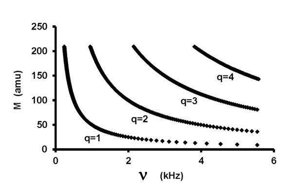 |
Fig.(1). M vs. v , Eq. (6). |
Fig. (2) shows the number of mass numbers within a ± 2% frequency window as a function of frequency according to Eq. (7) [obtained by differentiating Eq. (6)], with .
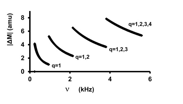 |
Fig.(2). |ΔM| in a ±2% frequency window vs. v, Eq. (7). |
Again, S = 1 μm. The discontinuities are the result of sequential addition of q-values from 1 to (1 and 2) to (1 and 2 and 3) to (1 and 2 and 3 and 4) with increasing frequency.
From Figs. (1 and 2) it is apparent that there are multiple choices of isotopic masses to satisfy Eq. (2) within a ±2% frequency window and that the number of choices increases with increasing frequency. This demonstrates the need for very complete and highly sensitive chemical analyses to guide interpretation. In this work, the (arbitrary) ±2% frequency window was met for 195 of 238 experimental frequencies. Better fits were possible in some cases, but only by introducing unlikely elements as impurities. Only about a fourth of all elements are "common," which constrains realistic assignments.
(6) Previous elastic mode interpretations of some of the audiofrequency resonances in lead, 2S Aluminum and in Teflon® failed to predict all the frequencies and no more. In these cases the particle wave theory predicted all the nonelastic frequencies (including overlaps with elastic frequencies) and no more. Only in the alnico samples did elastic theory predict all the frequencies (but only 2 in each of 2 samples) and no more in the frequency range of the experiment, but even here some frequencies were apparently discarded.
CONCLUSION
The following conclusions are drawn from the present work and careful reading of previously reported work:
- The Particle Wave Theory of plastic deformation in crystalline solids has been upheld by detailed quantitative interpretations of past MRD spectra of 38 samples obtained by six different research individuals or groups operating independently with seven different apparati.
- In larger samples, elastic normal modes are found in the audiofrequency range, where they occasionally overlap particle wave frequencies. Alternate interpretations according to various elastic theory expressions are either partially coincidental and inadequate as shown here or flawed as suggested by Fitzgerald [21].
- In addition to atoms and monatomic ions, interpretation of some spectra requires that molecules or molecular ions be proposed, especially for very low frequency resonances, necessitating a high mass particle (Eq. 2).
- In complex, multiphase systems such as some alloys, multiple crystal mosaic sizes, S, corresponding to different phases, are necessary to interpret the spectra. This applies in particular to precipitation hardened alloys.
- Fitzgerald's requirement that for particles to emerge in the field-free region they must be aligned in a row of evenly spaced like isotopes [8], seems unnecessary. The large number of isotopes and impurities in some materials and the imposition of maximum entropy (which favors mixing over segregation) make this segregation improbable or impossible. In fact, a simple particle-in-a-box model, without reference to a lattice, would appear to suffice for the interpretation of MRD spectra. This would also allow for a particle-wave interpretation of spectra of some amorphous or only slightly ordered structures with lengthy, open, field-free regions.
- The overall simplification of spectra with time, with increased static stress, and with annealing suggests that, under the influence of periodic shear stress, impurities move out of the primary phase into precipitates, dislocations, or grain boundaries. In this view, the odd substituent or interstitial atom would be more likely to enter the field free region because it would be out of phase (and hence in a higher energy state) with lattice vibrations, due to its different mass.
RECOMMENDATIONS FOR FUTURE WORK
Recommendations are made for future experiments in MRD:
- Repeat many of the original experiments on the same materials, this time analyzed for impurities by the current best techniques, including electron microprobe analysis (also see (3)). Keep sample size small enough to prevent interference from natural (elastic) frequencies. Measure higher frequencies (to 10 kHz or more) [40] to confirm assignments (same element, higher q-value). Always measure a no load or minimum load spectrum for comparison with other results and to complete the analysis in (5) below.
- Measure the resonance spectra of some materials with exchangeable cations, such as clays, zeolites, and ion exchange resins. Replace the ions and redetermine the spectra to see if frequencies shift predictably, i.e., v2/V1 = m1/m2 for masses m1 of original ion and m2 of replacement ion. We will then know for certain the origin of both frequencies.
- Integrate modern microscopy techniques on the same samples to determine distribution of impurities, their composition, and crystal mosaic size, before and after prolonged periodic stressing.
- Measure complete spectra in far less time than was required in the past (minutes instead of days or weeks) employing, for example, a more recent apparatus such as described in [40]. If equilibration is slow, this may not be possible, but it would open the possibility of studying the dynamics of equilibration.
- With (1) - (4) in hand, do more detailed time studies on changing samples to determine the fate of impurity particles under periodic stress (e.g., do they migrate to dislocations or grain boundaries, and do they form separate phases?). The application of periodic audiofrequency stress is a potential means of strengthening materials and otherwise affecting their properties, because it affects the distribution of impurities.
- Investigate amorphous and partially ordered materials, including quasi-crystals, to determine whether crystallinity is an absolute requirement for particle wave resonances.
- Confirm and explain the release of P atoms in bone apatite and Si and other atoms in quartz where they are tightly bonded to four oxygen atoms.
- Investigate the interaction of electromagnetic induction and radiation with solids exhibiting mechanical resonance dispersion. Potentially this could lead to detection and identification of materials at great distances, up to km. Further, because of its long wavelength, radiation in this audiofrequency region penetrates all common materials except metals, yielding opportunities for detection of hidden objects.
CONFLICT OF INTEREST
The author confirms that this article content has no conflict of interest.
ACKNOWLEDGEMENTS
Declared none.